Model Card for Neuropathology Vision Transformer: NP-TEST-0

This model is a Vision Transformer adapted for neuropathology tasks, developed using data from the University of Kentucky. It leverages principles from self-supervised learning models like DINOv2.

This model serves as an initial test while a proper training and evaluation dataset is generated

Model Details

Model Type: Vision Transformer (ViT) for neuropathology.
Developed by: Center for Applied Artificial Intelligence (CAAI)
Model Date: 05/2025
Base Model Architecture: Dinov2-giant (https://huggingface.co/facebook/dinov2-giant)
Input: Image (224x224).
Output: Class token and patch tokens. These can be used for various downstream tasks (e.g., classification, segmentation, similarity search).
Embedding Dimension: 1536
Patch Size: 14
Image Size Compatibility:
- The model was trained on images/patches of size 224x224.
- The model can accept images of any size, not just the 224x224 dimensions used in training.
License: Apache 2.0

Intended Uses

This model is intended for research purposes in the field of neuropathology.

Primary Intended Uses:
- Classification of tissue samples based on the presence/severity of neuropathological changes.
- Feature extraction for quantitative analysis of neuropathology.

Training Data

Dataset(s): The model was trained on data from the University of Kentucky.
- Name/Identifier: UK Alzheimer's Disease Center Neuropathology Whole Slide Image Cohort [BDSA TEST v1.0]
- Source: UK-ADRC Neuropathology Lab at the University of Kentucky University of Kentucky
- Description: The dataset contained 57 hole slide images (WSIs) of human post-mortem brain tissue sections. Sections were stained with Hematoxylin and Eosin (H&E).
- Preprocessing: WSIs were tiled into non-overlapping 224x224 pixel patches at multiple magnification levels (40x, 10x, 2.5x, and 1.25x). For each magnification level, a maximum of 1000 tiles per annotation label were extracted to ensure balanced representation across pathological features.
- Annotation : "Regions of interest (ROIs) for Gray Matter, White Matter, Leptomeninges, Exclude and Superficial Cortex were annotated. Annotations completed by Allison Neltner using a web-based tool developed my Thomas Pearce, MD (UMPC).

Training Procedure

Training System/Framework: DINO-MX (Modular & Flexible Self-Supervised Training Framework)
Training Infrastructure: 4 x DGS H100 nodes (32 x H100 GPUs)
Base Model (if fine-tuning): Pretrained facebook/dinov2-giant loaded from Hugging Face Hub.
Training Objective(s): Self-supervised learning using DINO loss, iBOT masked-image modeling loss.
Key Hyperparameters (example):
- Batch size: 32
- Learning rate: 1.0e-4
- Epochs/Iterations: 5000 Iterations
- Optimizer: AdamW
- Weight decay: 0.04-0.4

Evaluation

Task(s): Classification, KNN, Clustering, Robustness
Metrics: Accuracy, Precision, Recall, F1
Dataset(s): Neuro Path dataset
Results: The model achieved strong performance across multiple evaluation methods using the Neuro Path dataset.

Linear Probe Performance:
- Accuracy: 80.17%
- Precision: 79.20%
- Recall: 79.60%
- F1 Score: 77.88%
K-Nearest Neighbors Classification:
- Accuracy: 83.76%
- Precision: 83.34%
- Recall: 83.76%
- F1 Score: 83.40%
Clustering Quality:
- Silhouette Score: 0.267
- Adjusted Mutual Information: 0.473
Robustness Score: 0.574

Overall Performance Score: 0.646

Model Comparison

Models Evaluated

NP-TEST-0: Our model
dinov2-giant: Pretrained Dinov2 Giant
dinov2-giant_distilled_prov: Dinov2 Giant distilled from provo-gigapath
dinov2-large_distilled_prov: Dinov2 Large distilled from provo-gigapath
distilled_prov_finetuned: dinov2-giant_distilled_prov was used as a base with additional finetuning without freezing teacher model.
prov-gigapath: prov-gigapath/prov-gigapath
UNI: MahmoodLab/UNI
UNI2-h: MahmoodLab/UNI2-h

Linear Probe Comparison

Model	Accuracy	F1	Precision	Recall
NP-TEST-0	0.802	0.779	0.792	0.796
dinov2-giant	0.667	0.648	0.669	0.667
dinov2-giant_distilled_prov	0.769	0.756	0.755	0.769
dinov2-large_distilled_prov	0.772	0.758	0.758	0.772
distilled_prov_finetuned	0.779	0.762	0.770	0.779
prov-gigapath	0.776	0.762	0.764	0.776
UNI	0.741	0.731	0.734	0.741
UNI2-h	0.768	0.750	0.753	0.768

While the evaluation dataset was distinct from the training set, they were from the same institution, using the same staining, and obtained from the same scanner. It is not unexpected that a model fine-tuned on such a closely associated dataset would perform better. An evaluation dataset with broader representation is needed for a proper evaluation of generalized performance.

Model Evaluation Details

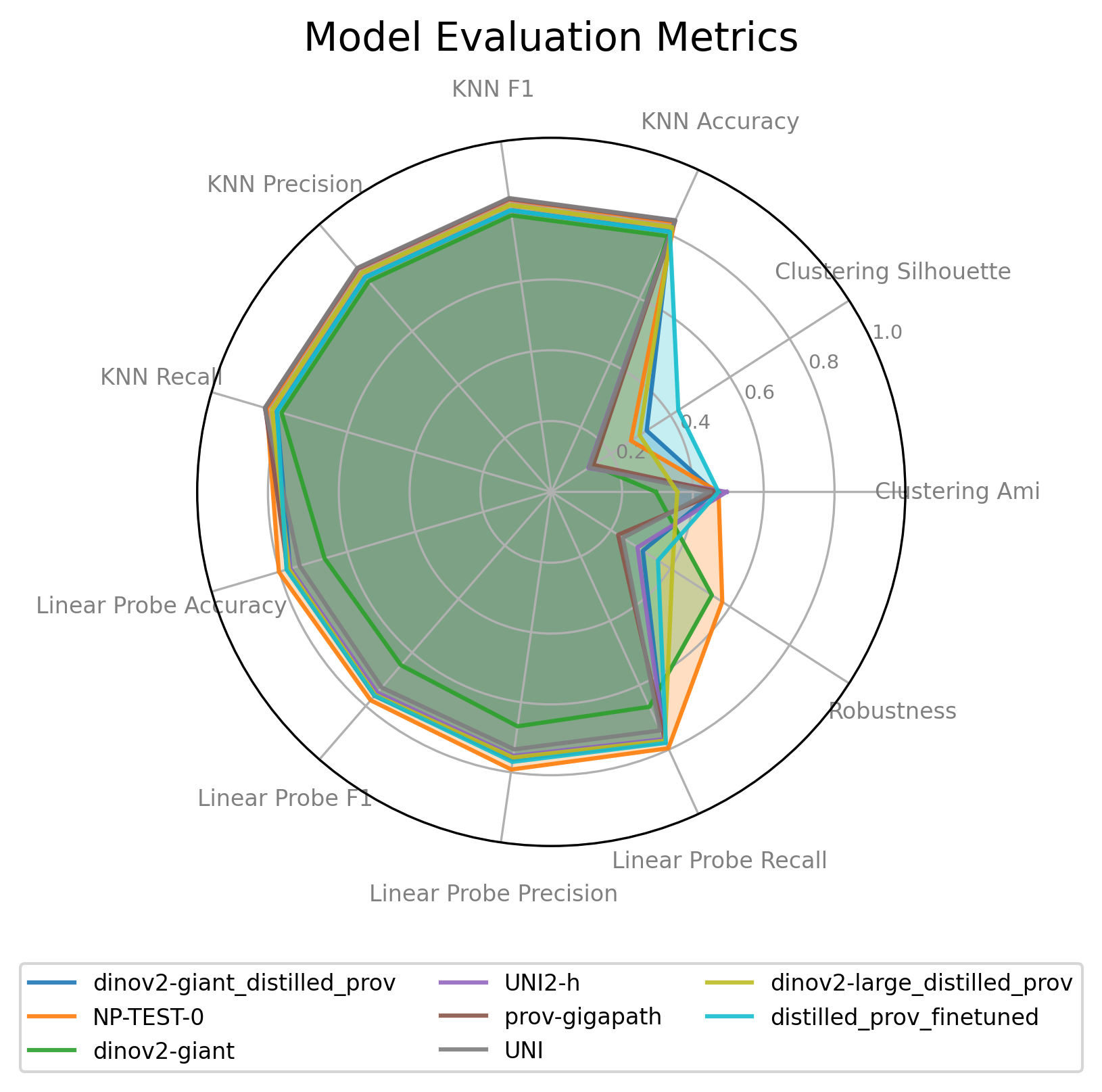
The radar chart provides a visual comparison of multiple models across several performance metrics. Each axis extending from the center represents a different metric. The farther a model's line is from the center along a particular axis, the better its score for that specific metric (assuming higher is better for the metric).

How to Interpret:

Axes: Each spoke of the radar represents a distinct evaluation metric.
Lines/Polygons: Each colored line (forming a polygon) represents a different model.
Performance: A point on an axis closer to the outer edge indicates a higher score for that metric.
Overall Comparison: By comparing the shapes and sizes of the polygons, you can get a quick visual understanding of the strengths and weaknesses of each model relative to others. A larger overall polygon generally suggests better all-around performance on the displayed metrics.

Tests

1. Linear Probe

What it is: This test evaluates the quality of the model's learned features (embeddings). A simple linear classifier is trained on top of these frozen features to perform a classification task.
Purpose: It assesses how well the learned representations can be used for downstream tasks with a minimal amount of additional training. Good performance indicates that the embeddings are linearly separable and capture meaningful information.
Metrics: Accuracy, Precision, Recall, F1-Score (calculated for the linear classifier).

2. K-Nearest Neighbors (KNN) Evaluation

What it is: This test also evaluates the quality of the model's embeddings. Instead of training a new classifier, it uses the K-Nearest Neighbors algorithm directly on the embeddings to make predictions. For a given data point, its class is determined by the majority class among its 'k' closest neighbors in the embedding space.
Purpose: It assesses the local structure and similarity relationships within the embedding space. Good KNN performance suggests that similar items are close to each other in the learned representation.
Metrics: Accuracy, Precision, Recall, F1-Score (calculated for the KNN classifier).

3. Clustering

What it is: This set of tests evaluates how well the model's embeddings can naturally group similar items together without predefined labels (unsupervised). Algorithms like K-Means are often used to partition the data points based on their embeddings.
Purpose: It assesses the intrinsic structure and separability of the learned representations into meaningful groups.
Common Metrics:
- Silhouette Score: Measures how similar an object is to its own cluster compared to other clusters. Ranges from -1 to 1 (higher is better).
- Adjusted Mutual Information (AMI): Measures the agreement between true labels (if available) and clustering assignments, adjusted for chance. Ranges from 0 to 1 (higher is better).

4. Robustness

What it is: This is a general category of tests designed to measure how well a model maintains its performance when faced with various challenges or changes in the input data.
Purpose: It assesses the model's stability and reliability under non-ideal conditions.
Examples of Challenges: This can include noisy data, adversarial attacks (inputs intentionally designed to fool the model), out-of-distribution samples (data different from what the model was trained on), or other perturbations.
Common Metrics: Often a "Robustness Score" is reported, which could be an accuracy, F1-score, or other relevant metric evaluated on the challenged dataset. The specific calculation depends on the nature of the robustness test. (Higher is generally better).

How to Get Started with the Model

Three example methods using Hugging Face transformers (adjust based on your actual model and task):


import torch
from PIL import Image
from transformers import AutoModel, AutoImageProcessor
from torchvision import transforms

def get_embeddings_with_processor(image_path, model_path):
    """
    Extract embeddings using a HuggingFace image processor.
    This approach handles normalization and resizing automatically.
    
    Args:
        image_path: Path to the image file
        model_path: Path to the model directory
        processor_path: Path to the processor config directory
    
    Returns:
        Image embeddings from the model
    """
    # Load model
    model = AutoModel.from_pretrained(model_path)
    model.eval()
    
    # Load processor from config
    image_processor = AutoImageProcessor.from_pretrained(model_path)
    
    # Process the image
    with torch.no_grad():
        image = Image.open(image_path).convert('RGB')
        inputs = image_processor(images=image, return_tensors="pt")
        outputs = model(**inputs)
        embeddings = outputs.last_hidden_state[:, 0, :]
    
    return embeddings

def get_embeddings_direct(image_path, model_path, mean=[0.83800817, 0.6516568, 0.78056043], std=[0.08324149, 0.09973671, 0.07153901]):
    """
    Extract embeddings directly without an image processor.
    This approach works with various image resolutions since transformers handle
    different input sizes by design.
    
    Args:
        image_path: Path to the image file
        model_path: Path to the model directory
        mean: Normalization mean values
        std: Normalization standard deviation values
    
    Returns:
        Image embeddings from the model
    """
    # Load model
    model = AutoModel.from_pretrained(model_path)
    model.eval()
    
    # Define transformation - just converting to tensor and normalizing
    transform = transforms.Compose([
        transforms.ToTensor(),
        transforms.Normalize(mean=mean, std=std)
    ])
    
    # Process the image
    with torch.no_grad():
        # Open image and convert to RGB
        image = Image.open(image_path).convert('RGB')
        # Convert image to tensor
        image_tensor = transform(image).unsqueeze(0)  # Add batch dimension
        # Feed to model
        outputs = model(pixel_values=image_tensor)
        # Get embeddings
        embeddings = outputs.last_hidden_state[:, 0, :]
    
    return embeddings

def get_embeddings_resized(image_path, model_path, size=(224, 224), mean=[0.485, 0.456, 0.406], std=[0.229, 0.224, 0.225]):
    """
    Extract embeddings with explicit resizing to 224x224.
    This approach ensures consistent input size regardless of original image dimensions.
    
    Args:
        image_path: Path to the image file
        model_path: Path to the model directory
        size: Target size for resizing (default: 224x224)
        mean: Normalization mean values
        std: Normalization standard deviation values
    
    Returns:
        Image embeddings from the model
    """
    # Load model
    model = AutoModel.from_pretrained(model_path)
    model.eval()
    
    # Define transformation with explicit resize
    transform = transforms.Compose([
        transforms.Resize(size, interpolation=transforms.InterpolationMode.BICUBIC),
        transforms.ToTensor(),
        transforms.Normalize(mean=mean, std=std)
    ])
    
    # Process the image
    with torch.no_grad():
        image = Image.open(image_path).convert('RGB')
        image_tensor = transform(image).unsqueeze(0)  # Add batch dimension
        outputs = model(pixel_values=image_tensor)
        embeddings = outputs.last_hidden_state[:, 0, :]
    
    return embeddings

# Example usage
if __name__ == "__main__":
    image_path = "test.jpg"
    model_path = "IBI-CAAI/NP-TEST-0" 
    
    # Method 1: Using image processor (recommended for consistency)
    embeddings1 = get_embeddings_with_processor(image_path, model_path)
    print('Embedding shape (with processor):', embeddings1.shape)
     
    # Method 2: Direct approach without resizing (works with various resolutions)
    embeddings2 = get_embeddings_direct(image_path, model_path)
    print('Embedding shape (direct):', embeddings2.shape)
    
    # Method 3: With explicit resize to 224x224
    embeddings3 = get_embeddings_resized(image_path, model_path)
    print('Embedding shape (resized):', embeddings3.shape)

Acknowledgements:

This initial work was supported by the broader Brain Digital Slide Archive (BDSA) Team.

This research was supported by the National Institute of Neurological Disorders and Stroke (NINDS) of the National Institutes of Health (NIH) under award numbers:

1U24NS133945 (Principal Investigator: Peter T. Nelson). Project Title: Federated digital pathology platform for AD/ADRD research and diagnostics.
1U24NS133949 (Principal Investigator: David Andrew Gutman). Project Title: Brain Digital Slide Archive: An Open Source Platform for data sharing and analysis of digital neuropathology.

Contact

For any additional questions or comments, contact CAAI ([email protected]), Mahmut Gokmen ([email protected]) Cody Bumgardner ([email protected]).

Citation / BibTeX

In process

IBI-CAAI
/

NP-TEST-0