Automatic Prompt Optimization with DSPy and Cross Encoders

Table of Contents
I recently trained a new set of cross encoders based on Ettin encoders from Johns Hopkins University. The encoders from this collection are based on ModernBERT, a BERT architecture that is updated for computationally efficient inference. While the original ModernBERT series only included base and large models, Ettin increased the number of sizes into much smaller sizes (as small as 17M parameters). How perfect for CPU inference!
To showcase one way you can use these models, I demonstrate one of my favorite applications -- evaluation and automated prompt optimization with DSPy. Say goodbye to the days of vibe-inferencing and start evaluating your AI programs. Bring LLMs back into the realm of machine learning in your projects.

Cross Encoders
Cross encoders are BERT models that take pairs of text as inputs and use a classifier head, typically for comparative classification. Common uses include STS (semantic textual similarity), NLI (natural language inference) or reranking for retrieval. Unlike embedding models, where you'd compute embeddings separately and then calculate similarity (eg using cosine similarity), cross encoders take both sentences as input and the transformer attention looks at both sentences simultaneously. The classifier head gives you the classification or score for the task.
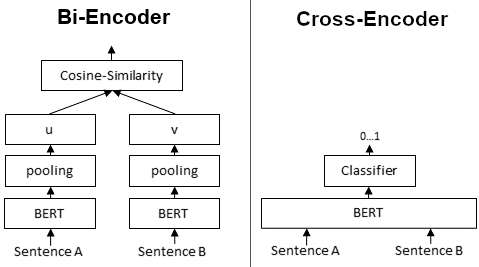
Cross encoders are usually trained for specific tasks. They tend to perform very well, but you'll pay for it with increased computational complexity (N^2 with token inputs and input sequences are doubled due to pairing). They also don't produce vectors you can store and reuse.
ModernBERT uses interleaved layers of local and global attention, and can handle longer inputs up to 8192 tokens. This makes it a good architecture for cross encoders. Local attention helps improve the efficiency by decreasing the size of the attention window, only using a few global attention layers, where necessary.
Cross Encoders as Evaluators
One of my favorite uses of cross encoders, especially STS models, is automated prompt optimization. STS models work great when you have natural language output, and you want to score the answer from an LLM (which may be correct but is worded differently). When you use them to evaluate LLM responses, you can see how well your prompt is performing. Then, using an optimizer like MIPROv2, you can synthetically generate better instructions, bootstrap examples and find good examples to add for few shot prompting.
DSPy Optimization
In this example, we'll load the HotPot QA dataset. This dataset might not see huge benefits in answer correctness, but we can still use our evaluator to guide how the LLM responds. For example, we can use examples to cause the outputs to be formatted similarly to our gold examples (the 'correct' answers from the dataset), and make sure prompt instructions are written well for the task. Optimization tends to work especially well for tasks where demo examples are really useful for improving performance (like classification, information extraction, etc).
Why DSPy?
If your goal is just to simplify writing code for inferencing an LLM, then there are a lot of options out there. However, when you first start DSPy, it's important to realize you're no longer learning an LLM framework, but a machine learning framework. This entails all of the usual suspects - evaluation, train/dev/test splits and optimization. When you bring this mentality into the world of AI application development, you'll soon realize that this is a familiar and well-trodden path: working with SMEs, evaluating your outputs, developing datasets and monitoring model performance.
When you start thinking this way, you'll realize many benefits:
- confidently switch between models (cost vs performance optimization)
- helps communicate the quality of your solution to the business
- enables monitoring for performance drift
- quit "prompt engineering" and get back to regular engineering
The hardest part is figuring out how to evaluate your outputs, which usually requires a bit of thought and creativity. There are many ways you can do this, for example LLM-as-a-Judge using another DSPy program. Or even more simply, using a cross encoder.
Setup the Evaluation Metric
First, we create a function that uses the cross encoder to provide an evaluation score between the golden example and the predicted example:
def cross_encoder_metric(cross_encoder_model, example, pred, trace=None):
    """Metric function using EttinX cross-encoder for semantic similarity evaluation"""
    gold_answer = example.answer.strip()
    pred_answer = pred.answer.strip() if hasattr(pred, 'answer') else str(pred).strip()

    sentence_pairs = [(gold_answer, pred_answer)]
    scores = cross_encoder_model.predict(sentence_pairs)
    similarity_score = float(scores[0])

    return similarity_score >= SIMILARITY_THRESHOLD if trace is not None else similarity_score
We use dleemiller/EttinX-sts-xs. This cross encoder is pretty small, and is plenty fast to run on CPU (I used it on my i5 laptop from 2019).
Load the Data
Now we need to load splits for the dataset. We use 3 splits train (used for demos, bootstrapping demos and proposing instructions),
dev (used for evaluating combinations of these things) and test (used for independently scoring before/after optimization).
def load_dataset(train_size=TRAIN_SIZE, dev_size=DEV_SIZE, test_size=TEST_SIZE):
    """Load HotPotQA dataset with specified splits"""
    console.log(f"Loading HotPotQA dataset (train:{train_size}, dev:{dev_size}, test:{test_size})")

    dataset = HotPotQA(
        train_seed=1, train_size=train_size,
        eval_seed=2023, dev_size=dev_size, test_size=test_size
    )

    # Set input keys as required by DSPy
    splits = {
        'train': [x.with_inputs('question') for x in dataset.train],
        'dev': [x.with_inputs('question') for x in dataset.dev],
        'test': [x.with_inputs('question') for x in dataset.test]
    }

    console.log(f"Loaded {len(splits['train'])} train, {len(splits['dev'])} dev, {len(splits['test'])} test examples")
    return splits['train'], splits['dev'], splits['test']
DSPy Signatures and Predictors
DSPy "signatures" are a lot like pydantic models, where you specify inputs and outputs. Of note, docstrings, field descriptions and type annotations are all important pieces of the "prompt" that is assembled. The docstring for the signature is effectively the "main prompt".
You will often see it written like this:
class QASignature(dspy.Signature):
    """Answer questions clearly and concisely"""
    question: str = dspy.InputField(desc="The question to answer")
    answer: str = dspy.OutputField(desc="The answer to the question")

predictor = dspy.ChainOfThought(QASignature)
Simple signatures can even use a shorthand:
predictor = dspy.ChainOfThought("question -> answer")
Though in practice, the former, more explicit declaration provides more flexibility. Once you add a predictor,
like dspy.ChainOfThought (for chain of thought responses), dspy.Predict (for simple prediction) or
dspy.ReAct (for agentic tool use), you can already start inferencing the LLM.
Training a DSPy Program
Setting up the training is fairly simple. There's a few parameters to set:
teleprompter = MIPROv2(
    metric=metric,
    auto="light",  # Can be "light", "medium", or "heavy"
    num_threads=1,
    verbose=True
)

optimized_program = teleprompter.compile(
    student=initial_program,
    trainset=trainset,
    valset=devset,
    requires_permission_to_run=False,
)
How MIPROv2 Works
MIPROv2 runs in three phases to systematically optimize your program.
Phase 1: Bootstrap Examples - Runs your program many times on training data, keeping only the input/output pairs that score well with your metric. This creates a pool of high-quality few-shot examples that actually work.
Phase 2: Generate Instructions - Creates multiple instruction variations by analyzing your training data patterns, program structure, and the bootstrapped examples. It adds random "tips" like "be creative" to explore different instruction styles.
Phase 3: Bayesian Search - Here's the key: your training set is only used for phases 1 and 2. Your validation set is used exclusively for evaluation during optimization. Bayesian optimization tests different combinations of instructions + few-shot examples, learning which combinations work well together rather than just trying random combos.
The result is a program where each predictor gets the best combination of instruction and examples that work together for your specific task and data.
Results
Here's how our optimization performed on the HotPot QA dataset. Starting with a simple predictor using basic instructions, MIPROv2 systematically improved performance through its optimization process.
Optimization Progress:
The optimization ran through 10 trials, testing different combinations of instructions and few-shot examples:
- Trial 1 (Baseline): 45.02% - Default program with basic instruction "Answer questions with step-by-step reasoning"
- Trial 2: 50.67% - Better performance with more detailed expert system instruction
- Trial 6: 60.52% - Best performance achieved by returning to the simple instruction but with optimized few-shot examples
- Final trials: Continued exploration but no further improvements found
Final Performance:
Performance Comparison
┏━━━━━━━━━━━━━━━━━━━━━━┳━━━━━━━━━┓
┃ Metric               ┃   Score ┃
┡━━━━━━━━━━━━━━━━━━━━━━╇━━━━━━━━━┩
│ Initial Program      │ 36.75   │
│ Optimized Program    │ 43.52   │
│ Improvement          │ +6.77   │
│ Relative Improvement │ +18.42% │
└──────────────────────┴─────────┘
Example Improvements:
Looking at specific examples, we can see how the optimization changed different types of questions:
- Answer format: The optimized model learned to give more concise answers (short response vs. full sentence explanation)
- Multi-hop reasoning: Adds useful chain-of-thought reasoning demos into the prompts.
The 18.42% relative improvement shows that even on a challenging multi-hop reasoning dataset like HotPot QA, systematic optimization is simple, effective and quantifies performance gains without having to manually adjust prompts.
Note: semantic similarity is not the same as correctness; however, it can work well for improving the consistency in your responses and is typically well correlated with correctness. STS works well in conjunction with LLM-as-a-judge as a more complete evaluation metric, by adding a fast, stable signal indicating topical/lexical alignment.
Conclusions
That's it! With a few simple steps, we set up evaluation and used it to actually optimize our program. We saw a solid improvement in our outputs, and many applications can see even bigger wins when N-shot examples really help the task.
Takeaways:
- Cross-encoders can be used as evaluators for semantic similarity tasks where exact string matching fails
- DSPy's systematic approach beats manual fiddling - Prompt engineering is time consuming and annoying without evaluations. MIPROv2 found combinations that would have taken a lot of poking and hoping.
- Small models work surprisingly well - the 32M parameter EttinX extra small model ran fast on CPU while giving reliable evaluation
- Proper ML practices matter - train/dev/test splits and systematic optimization make a real difference, and end up becoming time savers over the long run.
This scales well past toy examples. For production apps, you can use bigger validation sets, run more optimization trials, and mix multiple evaluation metrics. The framework gives you a solid base for building measurable AI systems you can actually trust to deploy.
I hope you got something out of this walkthrough and are inspired to take a systematic approach to prompt optimization in your own projects.
The full script for this blog can be found here: https://github.com/dleemiller/auto-prompt-opt-dspy-cross-encoders